Executing your Action or Activity Diagram

Introduction to executing an Action or Activity Diagram.

In the Action or Activity Diagram, users can execute their functional models with the Discrete Event or Monte Carlo Simulators, as highlighted above. Let's delve into an introductory explanation on setting up a functional model and utilize the scripting and distributions options provided in these diagrams. 

 

Introduction to Scripting Options

When selected, all Action Constructs in both the Activity or Action Diagrams have a 'Script' button appear on the top of the Toolbar Frame.

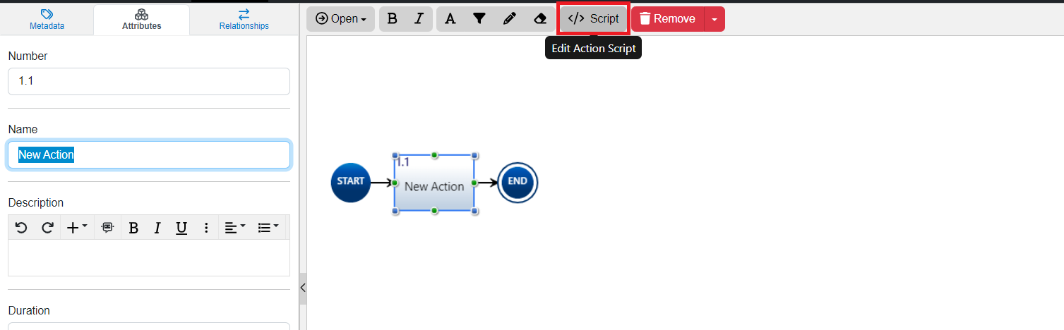This 'Script' button is a pop up to allow users to add JavaScript into their models for execution in the Simulator. This Script field is available for all Action constructs.

Depending on the specific type of Action construct selected, this popup can change to reflect options for that specific construct. Below we will cover these options provided per construct.

Loop Construct

The Script pop up for a Loop action defaults to the Iterations option. Here, users can select how many times to iterate the actions in the loop.

Note, the Loop Iterations field (circled in red above) is a dropdown and more options are provided to modify the behavior of the loop in the model. These options are shown below.

If Loop Probability is selected, the pop up will be changed to reflect percentage fields for users to select the probability of the loop continuing or exiting, as shown below. 50% is the default option for both options. Users may enter or use the selector that appears on the right by the percentage sign to enter their desired percentage.

A Loop Action can also be dependent on Resources. Once the Loop Resource option is selected, the Resource must be selected on the second dropdown, as shown in the image below.

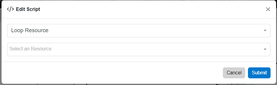
Once a Resource is selected, users will have to select the operator type, to continue the loop, based on the amount on the field on the right of the Continue Condition Dropdown. Operator Types included are Greater Than or Equal to, Greater Than, Less Than or Equal To, Less Than, or Equal To.

Underneath all these GUI options, is the JavaScript which is shown below, for 30 iterations. Not only will the 'Script' option reflect any of the options discussed above, but is also available for further editing to execute the model, by selecting 'Edit Script.'

OR Construct Script Options

The OR Construct's Script pop up defaults to the Probability option as shown above (if more branches are add the pop up will reflect the amount of branches available). Since the specific construct is an OR action, users may select how often, based off of a percentage, to go on to a particular branch. The Or construct can also be based off of a Resource, as shown below.

When the 'Or Resource' option is selected, the pop up will provide a second dropdown field to allow users to select a specific resource for the action to be dependent on.

Once this is selected, users may select the conditions of the resource for each branch. 

The conditions that can be set for each branch are shown below. They are Greater Than or Equal to, Greater Than, Less Than or Equal To, Less Than, Equal To, or Else.

Distributions

Distributions are vital in making a computer model more accurately represent a real-world system. Innoslate natively supports eight continuous distributions (Beta, Exponential, Gamma, Log-Normal, Normal, Triangular, Uniform, and Weibull) and two discrete distributions (Binomial and Poisson). Any of these distributions can be used in place of a simple value in any attribute of an entity or relationship which is of the data type 'Number' in your project’s database schema.

During a simulation run, Innoslate will use the distribution on an attribute to generate a random number for that attribute that falls within the bounds of the distribution. For example, when using a Uniform distribution where a = 15 and b = 20, the simulator could return a value of 16.835 in the first simulation run and a value of 19.015 in the second simulation run.

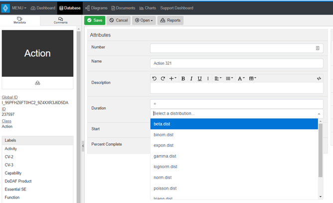
Adding a Distribution

Distributions can be added to any attribute of Number or Duration type, such as an Action class’s Duration or the Initial, Minimum, or Maximum Amount of a Resource. To add distribution to an attribute just start by typing in an “=”.  You will see a drop-down list of the supported distributions appear that you can select from.

 

More information on each of the supported distributions including parameters and common uses can be found below.

Continuous Distributions

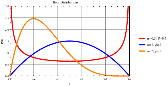
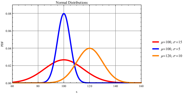
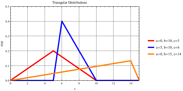
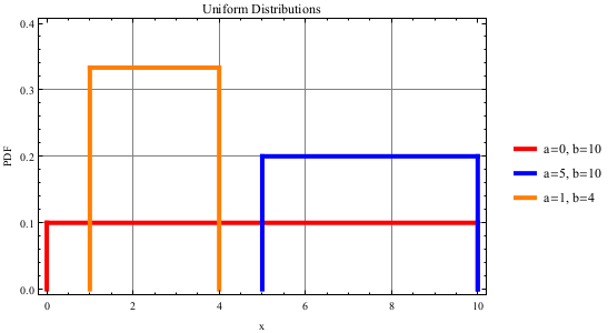
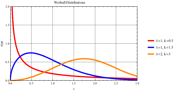
Each distribution has a plot of the distribution with multiple parameter options shown. The plot has an x value along the horizontal axis and the associated Probability Density Function (PDF) along the vertical axis. A higher PDF implies there will be a larger concentration of random numbers which fall within a given x range. Information on calculating the probability of a random number falling within a given range can be found at: http://en.wikipedia.org/wiki/Probability_density_function

During simulation Innoslate will return a random real value, x, such that a set of the values when plotted as a histogram will produce a shape nearing the shape of the distribution.

Beta Distribution

The Beta distribution is useful for generating a continuous random distribution between the fixed bounds of 0 and 1. The Beta distribution is best for predicting probabilities, calculating failure rates, or time allocation. For more information, see http://en.wikipedia.org/wiki/Beta_distribution.

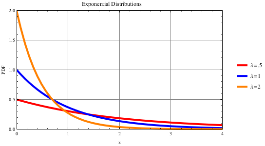
Exponential Distribution

The Exponential distribution describes the time intervals between a Poisson process. The return value, x, returns the next random interval between Poisson events. The Exponential distribution is best for describing the time between customer arrivals, service times, or time until the next particle decay. For more information, see http://en.wikipedia.org/wiki/Exponential_distribution.

Gamma Distribution

The Gamma distribution has many different uses including modeling the time required for k events to occur in a Poisson process, modeling waiting times, or resource consumption. For more information, see http://en.wikipedia.org/wiki/Gamma_distribution.

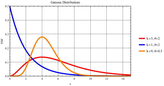
Note the Gamma distribution has two common formats. Innoslate uses the format of Gamma(k, θ) where k is the shape and θ is the scale. The second format is Gamma(α, β) where α is the shape and β is the rate. This second format can be transformed into the first format using the following equations: k = α, θ = 1/β

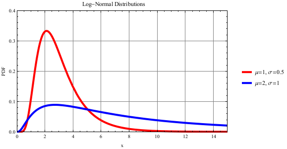
Log-Normal Distribution

The Log-Normal distribution generates a number equal to eN(μ, σ), where N(μ, σ) is a Normal distribution. The Log-normal distribution is best for describing the volume of gas in a reserve, incubation periods, or system repair time. For more information, see http://en.wikipedia.org/wiki/Log-normal_distribution.

Normal Distribution

The Normal distribution returns a value that will 95% of the time fall within 2 standard deviations (σ) of the mean (μ). This distribution is best for modeling natural processes, task completion time, or randomness of characteristics. For more information, see http://en.wikipedia.org/wiki/Normal_distribution.

Triangular Distribution

The Triangular distribution is best used when a minimum, maximum, and most likely outcome are known; providing basic randomness; or early estimation of task completion time. For more information, see http://en.wikipedia.org/wiki/Triangular_distribution.

Uniform Distribution

The Uniform distribution is commonly used in risk analysis, to calculate an unknown wait time, or randomly choose a selection in a set. For more information, see http://en.wikipedia.org/wiki/Uniform_distribution_(continuous).

Weibull Distribution

The Weibull distribution is a very versatile distribution, with the ability to be right-skewed, left-skewed, or symmetric. Due to this ability, the Weibull distribution is often used to model component reliability or characteristics, an increase or decrease in capability, or a system’s lifetime. For more information, see http://en.wikipedia.org/wiki/Weibull_distribution.

Discrete Distributions

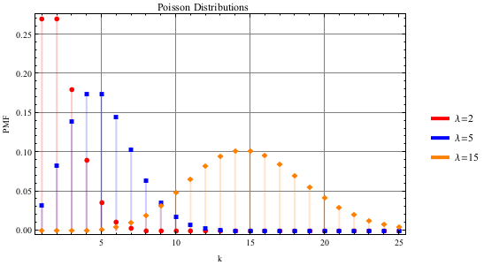
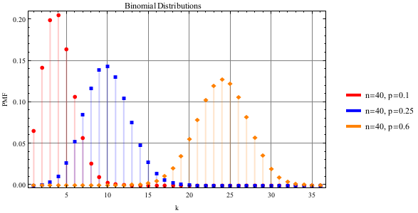
Each distribution has a plot of the distribution with multiple parameter options shown. The plot has a k value along the horizontal axis and the associated Probability Mass Function (PMF) along the vertical axis. A higher PMF implies there will be a larger concentration of random numbers which fall on a specific value. Information on calculating the probability of a random number falling within a given range can be found at: http://en.wikipedia.org/wiki/Probability_mass_function

During simulation Innoslate will return a random whole value, k, such that a set of the values when plotted as a bar graph will produce a shape nearing the shape of the distribution.

Binomial Distribution

The Binomial distribution models the number of successes from n independent trials where there is the same probability p of success in each trial. The Binomial distribution is best for counting the number of part failures based on n attempts, the number of failures generated from a repeated process, or the number of successful transmissions between wireless devices. For more information, see http://en.wikipedia.org/wiki/Binomial_distribution.

Poisson Distribution

The Poisson distribution models the number of events occurring over an interval of time, where λ is the mean number of events in that interval. Common uses of the Poisson distribution include counting the number of arrivals per day, ideal vehicle distance in traffic flow, or counting the number of resources needed to be consumed. For more information, see http://en.wikipedia.org/wiki/Poisson_distribution.