Innoslate Help Center

Getting Started

Platform Walkthrough

Model-Based Systems Engineering

This guide demonstrates how to use Innoslate for Model-Based Systems Engineering and builds upon the “Lesson – Autonomous Vehicle” project used in the previous guide.

Welcome to the Model-Based Systems Engineering guide!

This guide demonstrates how to use Innoslate for Model-Based Systems Engineering and builds upon the “Lesson – Autonomous Vehicle” project used in the previous guide. If you haven’t already, we recommend reading our Requirements Management and Analysis guide before proceeding with this guide.

Mercedes-Benz-Autonomous-Concept-Car (1) Photo: Mercedes Benz

At its core, Innoslate is a full Model-Based Systems Engineering tool. According to the INCOSE SE Vision 2020, “Model-Based Systems Engineering (MBSE) is the formalized application of modeling to support system requirements, design, analysis, verification and validation activities beginning in the conceptual design phase and continuing throughout development and later life cycle phases.”

Within Innoslate, system models are formalized and capable of simulation to derive cost, schedule, and performance data. Continue to the next section to see this in action.

Functional Modeling

Functional modeling is at the heart of how Innoslate derives new requirements and ensures logical accuracy. You are probably familiar with flowcharts that depict processes or task sequences. Functional modeling is a means to create these flowcharts so that rules of logic are enforceable, and integrated performance information is derivable from these models. To begin your first functional model, follow the steps below:

Click the ‘Diagrams’ button on the top navigation bar to navigate to ‘Diagrams View.’
Click the ‘+ Create Diagram’ button to create a new diagram.
Select ‘Action Diagram’ under ‘LML Diagrams’ as your diagram type.
Click the ‘Next’ button.
Type in “Metafunction” for the name of your new diagram.
Click the ‘Finish’ button.

After opening the ‘Action Diagram,’ a Start and End vertex is displayed. At the highest level (root) Metafunction, each ‘Asset’ will operate on its own separate lifeline. In Innoslate's Action Diagram, this is expressed with the ‘Parallel’ construct. This allows each ‘Asset’ to operate and communicate via ‘Input/Output’ constructs independently. Utilize these three primary ‘Assets’ – “User,” “Autonomous Vehicle,” and “Environment” – to model the “Autonomous Vehicle.” To create this:

Drag the ‘Parallel’ icon over to the arrow line between the Start and End nodes.
Click the ‘Add Branch’ button located on the toolbar to add a branch to the ‘Parallel’ construct.
Drag the ‘Branch Asset’ icon over to the top branch of your newly added ‘Parallel.
Type in “User” for the name of your new ‘Branch Asset.’
Repeat steps 3-4 for the middle and bottom branches naming the assets “Autonomous Vehicle” and “Environment,” respectively.

With the parallel branches in place, we now need to add the primary actions for each ‘Asset.’ To create this:

Drag the ‘Action’ icon over to the “User” parallel branch.
Type in “Set a Destination” for the name of your new ‘Action.’
Click anywhere in the white space to deselect.
Drag the ‘Action’ icon over to the “Autonomous Vehicle” parallel branch.
Type in “Drive Vehicle” for the name of your new ‘Action.’
Click anywhere in the white space to deselect.
Drag the ‘Action’ icon over to the “Environment” parallel branch.
Type in “Exhibit Environmental Conditions” for the name of your new ‘Action.’

As described earlier, each parallel ‘Action’ must communicate through ‘Input/Output’ constructs. Two Input/Outputs “Destination Location” and “Environmental Conditions” which trigger “Drive Vehicle,” will be created. A trigger will block the execution of the ‘Action’ receiving the trigger until the ‘Action’ generating the trigger completes. Optional ‘Input/Outputs’ will allow the receiving ‘Action’ to execute immediately with or without the ‘Input/Output.’

To create these:

Click to select the generating ‘Action’ construct named “Set a Destination.”
Click and drag one of the green circles over to the receiving ‘Action’ construct named “Drive Vehicle” and release over the ‘Trigger’ option when the receiving ‘Action’ highlights green.
Name the new ‘Trigger’ “Destination Location.”
To create the second ‘Trigger,’ click to select the generating ‘Action’ construct named “Exhibit Environmental Conditions.”
Click and drag one of the green circles over to the receiving ‘Action’ construct named “Drive Vehicle” and release over the ‘Trigger’ option when the receiving ‘Action’ highlights green.
Name the second ‘Trigger’ “Environmental Conditions.”

We need to further decompose the model for the “Autonomous Vehicle.” We will now create a decomposition ‘Action Diagram’ by performing the following steps:

Within the “Metafunction” diagram, click to select the ‘Action’ construct named “Drive Vehicle.”
Click to open the ‘Open’ drop-down and select the ‘Decomposition Diagram’ menu item.

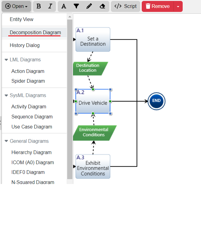
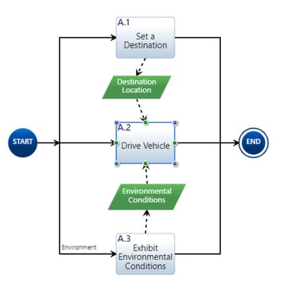
You will notice the ‘Input/Output’ constructs that are received and generated by “Drive Vehicle” are already placed on the diagram for convenience. The “Autonomous Vehicle” will need to loop until a destination is reached. During each iteration, the vehicle shall monitor the environment, calculate waypoints and obstacles, and navigate. “Camera” and “LIDAR” (‘Input/Outputs’) will transfer from the Sensors (‘Asset’), through the “Monitor the Environment” (‘Action’) to the “Control System” (‘Asset’). The control system will then calculate the waypoint and obstacles and transfer this data to the drive system. The drive system will then navigate the vehicle. We will construct this diagram (as we did with the “Metafunction” diagram) by drag-and-dropping from the left sidebar (as shown below in the “Drive Vehicle” diagram).

* Note: The direction of the dashed arrow lines drawn between the ‘Input/Output’ constructs and the ‘Action’ constructs is very important to get correct, otherwise the model may not be executable.

Use the table detailing the entities shown on the “Drive Vehicle” Action Diagram below to develop your model. The “Drive Vehicle” diagram includes a ‘Loop’ construct named “Reached Destination?” that will loop continuously until the final destination is reached.

* Note: The “Destination Location” and “Environmental Conditions” ‘Input/Output’ constructs are optional as these inputs are only generated once by the parent diagram. In order for a simulation to execute an ‘Input/Output’ completely, you must generate it for each iteration or mark it as optional.

Action Name	Inputs	Outputs	Branch Asset
Reached Destination? (Loop)	Destination Location (Optional)		N/A
Monitor Environment	Environmental Conditions (Optional)	Camera Data, LIDAR Data	Sensor
Calculate Waypoint and Obstacles	Camera Data (Trigger), LIDAR Data (Trigger), Destination Location (Optional)	Waypoint, Obstacles	Control System
Navigate Vehicle	Waypoint (Trigger), Obstacles (Trigger)		Drive System

We now need to elaborate on the functionality of the “Monitor Environment” action. Open the ‘Decomposition Diagram’ for “Monitor Environment.” Use the left sidebar to drag constructs to build the diagram below:

A table detailing the “Monitor Environment” entities follows. Note the ‘Input/Outputs’ will automatically display on the diagram from the parent level. This ensures ‘Input/Outputs’ are traced properly at lower levels.

Action Name	Inputs	Outputs	Branch Asset
Acquire LIDAR Data	Environmental Conditions (optional)	LIDAR Data	LIDAR
Acquire Camera Data	Environmental Conditions (optional)	Camera Data	Camera

Once you have completed the “Monitor Environment” diagram, we need to open the parent diagram named “Drive Vehicle.” To open the parent diagram:

Click on the ‘Open’ drop-down and select the ‘Parent Diagram’ menu item.

From the “Drive Vehicle” diagram we now need to open the “Calculate Waypoint and Obstacles” Decomposition Diagram to elaborate on its functionality. As before, use the left sidebar to drag constructs to build the diagram pictured below:

A table detailing the “Calculate Waypoint and Obstacles” entities follows.

Action Name	Inputs	Outputs	Branch Asset
Transform Images	Camera Data	Parsed Images	Main Computer
Parse for Obstacle Locations	Parsed Images	Obstacles	Main Computer
Convert LIDAR Data to Obstacles	LIDAR Data	Obstacles	Main Computer
Gather GPS Data		GPS Data	FPGA
Accelerate / Decelerate to Reach Speed Limit	GPS Data, Obstacles		FPGA
Update Waypoint	GPS Data, Destination Location (optional)	Waypoint	FPGA

Let’s Auto Number the entire hierarchy.

Click on the ‘Diagrams’ button on the top navigation bar to navigate to ‘Diagrams View.’
Open the ‘Action Diagram’ named “Metafunction.”
Click ‘Settings’ on the toolbar and select the ‘Auto Number’ menu item.
Type in “A” for the prefix.
Click the ‘Run’ button.

Let’s review the entire functional model using the ‘Hierarchy Chart.’ To open the ‘Hierarchy Chart’ for the root of the functional model:

From the “Metafunction” diagram, click to open the ‘Open’ drop-down.
Under the “General Diagrams” section, select the ‘Hierarchy Chart’ menu item.

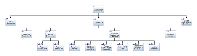
This ‘Hierarchy Chart’ was automatically generated from the ‘Action Diagram’ models we created. This chart displays the entire functional decomposition of ‘Action’ entities that we created earlier.

Physical Modeling

We can describe synthesizing the physical model in Innoslate with eight different diagrams, including the Asset Diagram, Layer Diagram, Block Definition Diagram, and Internal Block Diagram. In this section, we will focus on the Asset Diagram and Hierarchy Chart.

Earlier, we defined ‘Assets’ through modeling the Action Diagram; let’s now refine our physical model. In the Functional Modeling lesson, we created ‘Assets’ which perform ‘Actions’ that generate and receive ‘Input/Outputs.’ This information is used to automatically generate our physical diagrams. To begin:

Click the ‘Diagrams’ button on the top navigation bar to navigate to ‘Diagrams View.’
Open the ‘Action Diagram’ named “Metafunction.”
Click ‘Settings’ in the toolbar.
Select the ‘Generate Asset Diagram’ menu item.
This has generated our first Asset Diagram.

The ‘Asset Diagram’ describes the parts of the system represented as blocks and their connections shown as lines. Similar to Action Diagrams, Asset Diagrams are decomposable to further describe subordinate levels of the system.

To complete our physical model, we will repeat the steps above and generate Asset Diagrams using Asset Diagram Generation from the following decomposed Action Diagrams: “Drive Vehicle,” “Calculate Waypoint and Obstacles,” and “Monitor Environment.”

Let’s review our physical model with the ‘Hierarchy Chart.’ To open the ‘Hierarchy Chart’ for the root of the physical model, follow the steps below:

Click the ‘Diagrams’ button on the top navigation bar to navigate to ‘Diagrams View.’
Open the ‘Asset Diagram’ named “Metafunction (Physical Context).”
Click to open the ‘Open’ drop-down.
Under the “General Diagrams” section, select the ‘Hierarchy Chart’ menu item.

The physical hierarchy should appear as above. If your ‘Hierarchy Chart’ differs, ensure that all four Asset Diagrams were automatically generated (see above for steps to generate the Asset Diagrams).

Now, let’s Auto number the entire hierarchy.

From the hierarchy chart, click ‘Settings’ in the toolbar.
Select the ‘Auto Number’ menu item.
Type in “P” for the prefix.
Click on the ‘Run’ button.

With our full physical hierarchy created and related to our functional model, we will generate a ‘Block Definition Diagram (BDD).’ To generate a BDD:

Click on the ‘Open’ drop-down.
Under the “SysML Diagrams” section, select the ‘Block Definition Diagram’ menu item.

The BDD represents our physical hierarchy and its relationships to the functional model. Now that the primary entities of the executable model are completed, let’s execute the model.

Executing the Model

Innoslate includes a ‘Discrete Event Simulator’ to verify the Action Diagram logic, calculate the cost, compute time, and quantify performance. This simulation engine can run thousands of iterations in the ‘Monte Carlo Simulator’ to observe variance across many simulation runs. In this section, we will focus on simply running the simulation to verify logical correctness. A detailed simulation tutorials is available here.

To navigate to the ‘Discrete Event Simulator’ follow these instructions:

Click the ‘Diagrams’ button on the top navigation bar.
Open the ‘Action Diagram’ named “Metafunction.”
Click to open the ‘Simulate’ drop-down located on the toolbar.
Select the ‘Discrete Event’ menu item.

The Action Trace 3D panel displays the decomposed layers of our Action Diagram in a single 3D display. The Total Time and Total Cost panes display running totals for time and cost accordingly. Note that in this example, all durations default to 1 hour. Ideally, assign all Actions to a constant or distribution of time through the Duration attribute in every Action. Click the ‘Play’ button to begin the simulation.

As the simulation runs, a prompt will be displayed. Type in “10” for the number of loop iterations and click the ‘Submit’ button. The Status Panel records which Action is currently running or blocked for execution. The color of the progress bar in the Status pane indicates the current status. The same colors are used in the Action Trace 3D to indicate which Actions are currently queued.

Color	State	Description
Yellow	Input/Output Wait	The Action is waiting for an Input/Output(s).
Green	Executing	The Action is currently executing.
Blue	Complete	The Action has completed execution.

The table above shows applicable wait state colors for this example. The Gantt Chart displays the order of execution in a familiar format to project managers. This Gantt Chart is easily exported to Microsoft Project by clicking the "more" tab and selecting “Export to Project.”

After the simulation has run, reports are available to export to Excel for further analysis. Additional panes for Cost, Time, Resources, and General (ex. Console), as needed.

We have yet to trace our model to the original requirements.

To return to the ‘Action Diagram,’ click the ‘Innoslate’ button located below the Innoslate logo in the upper left-hand corner.

Relating Requirements to Diagrams

Requirements traceability ensures that the lifecycle and origin of a requirement are fully tracked. Innoslate includes relationship matrices to represent traceability relationships between entities in a tabular view.

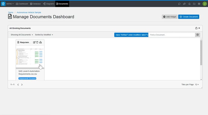
To open the requirements matrix:

From ‘Documents View,’ open the Requirements Document: “SAE Level-5 Automation Requirements.”
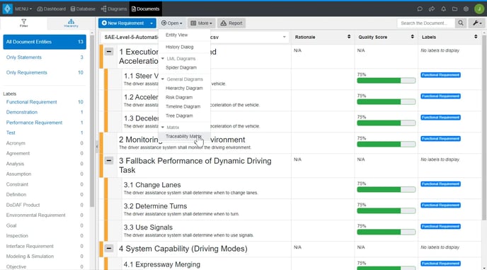
Click the ‘Open’ drop-down menu.
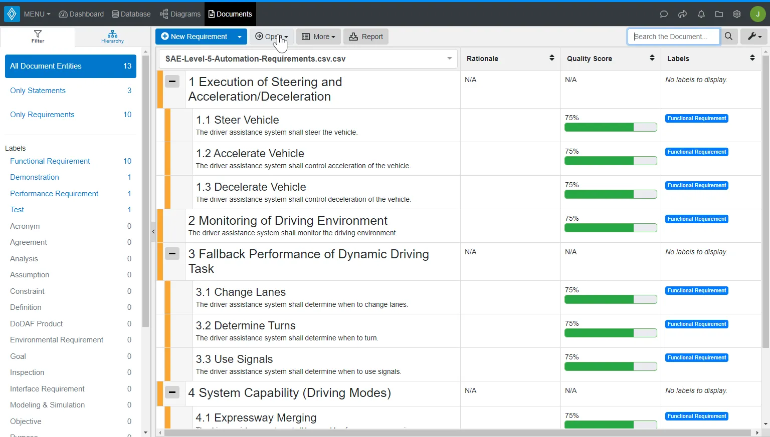
Click ‘Traceability Matrix’ under ‘Matrices.’
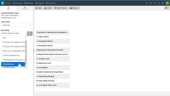
Ensure ‘Hierarchy’ is selected for the ‘Top (X Axis).’
Select ‘A Metafunction’ as the ‘Root Entity.’
Select ‘satisfied by’ as the ‘Relationship Type.’

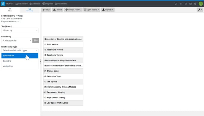
We are now viewing a matrix displaying the traceability between the requirements and the functional model we developed earlier.

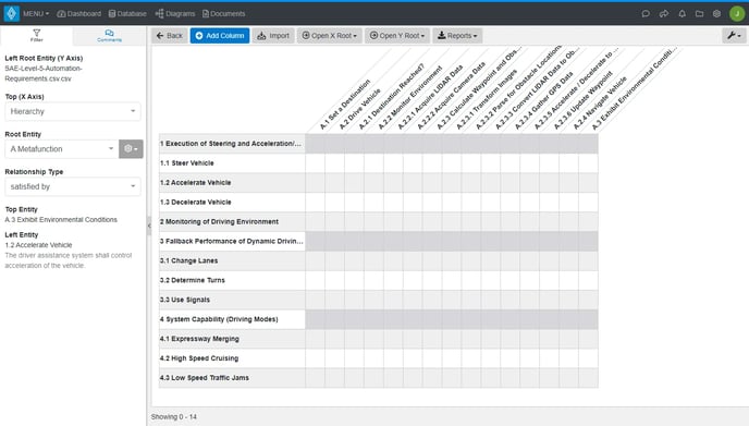
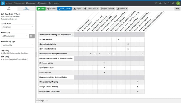
Note that traceability is not yet defined. To add a relationship, simply click the box in the cell between an Action and its associated requirement. These relationships express the traceability between the requirements and the functional model. Repeat this process until the matrix appears as below.

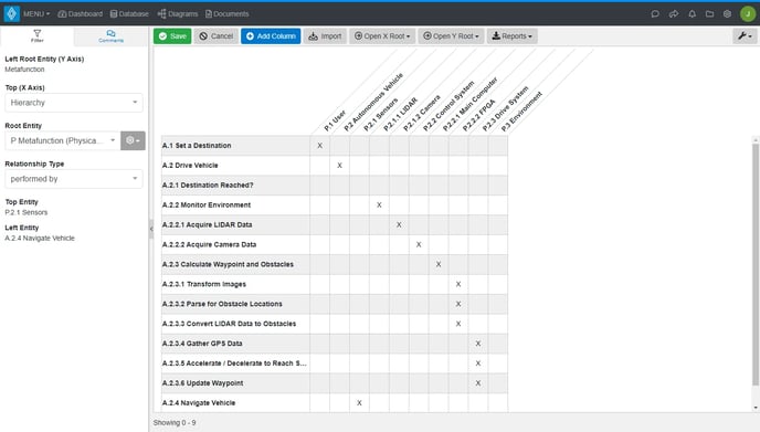
Matrices can display any relationship within Innoslate. For example, a matrix between “Metafunction” and “Metafunction – Physical Context” is displayed below using the ‘performed by’ relationship.

From ‘Diagrams View,’ open the Action Diagram “A Metafunction.”
Click the ‘Open’ drop-down menu.
Click ‘Traceability Matrix’ under ‘Matrices.’
Ensure ‘Hierarchy’ is selected for the ‘Top (X Axis).’
Select ‘P Metafunction (Physical Context)’ as the ‘Root Entity.’
Select ‘performed by’ as the ‘Relationship Type.’

Through this matrix, we will notice that “Reached Destination?” is not performed by any assets. Let’s add a ‘performed by’ relationship between “Autonomous Vehicle” and “Reached Destination?” by clicking the cell at their intersection.

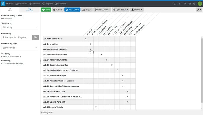
Click the ‘Save’ button to record the change.

Ensuring Overall Model Quality

As an Innoslate project grows in size and complexity, so does ensuring model quality. In the software domain, many tools exist to maintain quality: compilers, static code analysis tools, and even automatic graders. The value of these tools is increased accuracy and significantly reduced cost.

Innoslate includes three tools to ensure models developed are of high quality. The “Quality Check” feature of ‘Documents View’ is utilized to assess the quality of textual requirements, as covered earlier in the Requirements Management and Analysis guide. The simulators can validate the logic of a functional behavior model. ‘Intelligence’ analyzes the model to assess traceability, model construction, naming conventions, and more.

To run an ‘Intelligence’ analysis:

1. Open the ‘MENU’ drop-down and click the ‘Intelligence’ menu item under the “Tools” section.
2. Once in the ‘Intelligence’ tool, the analysis will begin automatically the first time you open the view. To re-run the analysis (after model changes), click on the ‘Run’ button.

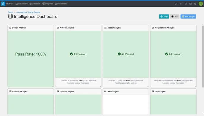
As you can see, Intelligence has analyzed our models using heuristics and machine learning language models. There are six sections assessed: “Global,” “Action,” “Asset,” “Conduit,” “Input/Output,” and “Requirement.” You will notice that the model we created receives a 100 percent in each category based on the default settings.

You may wish to enable additional checks or remove checks that are unimportant to your use case. To do this, click on the ‘Settings’ button on the top right to modify which checks are performed and their criticality (warning/error).