
Sections Available in Advanced Simulator Features
| Function | Description |
|---|---|
| Scripts | Explore the power of scripts, allowing you to automate and customize simulations over system behavior and event sequences through action entities. |
| Asset Utilization Over Time | Tracking Asset Utilization in the Simulator. |
| Capacity | How to utilize the Simulator to include throughput and latency. |
| Cloning | Understanding Action Cloning in the Simulator and its Behavior |
| Cost | Understanding how to track Cost in the Simulator. |
| Wait States | Insight into the Color Legend of the Discrete Event Simulator During Execution. |
Scripts
The simulator has three JavaScript functions, shown below, which are called during execution and can be overridden by the user to run custom scripts. A script can have one or all three of these functions in addition to any other helper functions necessary.
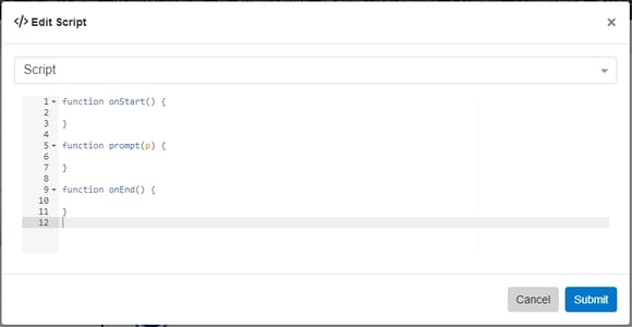
Each of these functions executes at a different time during the course of a construct being executed. The “onStart” function is executed after all the ‘Input/Output’ triggers have been completed but before any ‘Resource’ consumption and/or Asset utilization. The “prompt” function is executed after the ‘Resource’ consumption and/or Asset utilization but before the construct begins its Duration. The “onEnd” function executes after the construct’s Duration has ended.
Note: Any other functions must be called from within one of these three functions or they will not be executed by the simulator.
Scripting Prompts
Prompts allow the simulator to get input directly from the user. A prompt will cause the simulator to wait until input from the user has been received. Prompts are used in ‘OR’ and ‘LOOP’ constructs if no scripts are found and the simulator is in “Prompt Mode.” Prompts can be created by using one or more of these functions inside the “prompt” function. The title variable sets the title of the prompt. The name variable is the key that the response from the user will be stored under. The choices variable is the array of options for the user to choose from. The value variable is the default value entered in the prompt field. Below is a table of the types of prompts available to be scripted:
| Function | Description |
|---|---|
| addEnumInput(title, name, choices, value) | Prompts the user to choose from a set of predefined choices. |
| addTextInput(title, name, value) | Prompts the user to enter text. |
| addBigtitleTextInput(title, name, value) | Prompts the user to enter a large amount of text. |
| addNumberInput(title, name, value) | Prompts the user to enter a number. |
| addBooleanInput(title, name, value) | Prompts the user to choose from True or False. |
| setTitle(title) | Sets the title of the prompt. |
The “onEnd” function will receive the response from a scripted prompt in the form of a map. Below is an example of a simple prompt script that prompts for the user’s name and then prints their name from the response map to the web browser’s console within the “onEnd” function:

Simulator Scripting API
The simulator has a scripting API to allow users to gain access to data contained in the model being executed. The table below identifies each of the functions available in the API and what they return:
| Function | Description |
|---|---|
| Sim.getEntitiesByNumber(number) | Returns a list of entities based on the entity’s number. |
| Sim.getEntityByNumber(number) | Returns the first entity result based on the entity’s number. |
| Sim.getEntitiesByName(name) | Returns a list of entities based on the entity’s name. |
| Sim.getEntityByName(name) | Returns the first entity result based on the entity’s name. |
| Sim.get(name) | Short-hand alias for GetEntityByName. |
| Sim.getEntityById(id) | Returns an entity based on its id. |
| Sim.setResourceByName(name, amount) | Sets the resource’s current amount based on the resource’s name. |
| Sim.setResourceById(id, amount) | Sets the resource’s current amount based on the resource’s id. |
| Sim.getResourceByName(name) | Returns the first resource based on its name. |
| Sim.getAmount(name) | Returns the resource amount based on the resource’s name. |
| Sim.getAmountById(id) | Returns the resource amount based on the resource’s id. |
| Sim.getCurrentCost() | Returns the current cost of the simulation. |
| Sim.getIOValueByNumber() | Returns the Input/Output value attribute based on entity number. |
| Sim.getIOValueById() | Returns the Input/Output value attribute based on entity id. |
| Sim.getIOValueByGlobalId() | Returns the Input/Output value attribute based on entity global id. |
| Sim.getCurrentTime() | Returns the current time of the simulation. |
| Sim.httpGet(url) | Allows the user to do a synchronous GET request which will get data from an external server. |
| Sim.httpPost(url) | Allows the user to do a synchronous POST request which will create data on an external server. |
| Sim.httpPut(url) | Allows the user to do a synchronous PUT request which will update data on an external server. |
Controls
Innoslate offers additional simulator capabilities, which allow a user to further control and/or customize model execution. Below will cover those in more detail.
Asset Utilization Over Time
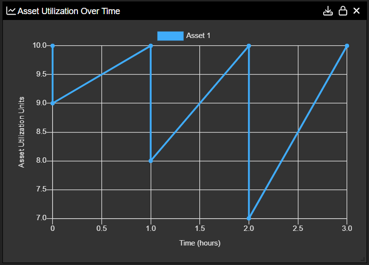
Asset Utilization prevents over-allocating a particular ‘Asset’ to an ‘Action.’ Asset Utilization will capture an ‘Asset’ once an ‘Action’ executes. The usage of each ‘Asset’ is monitored during the simulation and graphically displayed in the simulation results.
To control simulation flow, each ‘Asset’ utilized must have a parent ‘Asset.’ Typically, an Innoslate model will have a Physical Hierarchy of ‘Assets.’ ‘Assets’ in this hierarchy have a Multiplicity relationship attribute. If the ‘Asset’ is part of this hierarchy and the Multiplicity relationship attribute is set then the ‘Asset’ can be utilized. To utilize an ‘Asset,’ set the Amount attribute on the performed by relationship. In the simulation, if an ‘Asset’ is over-utilized then the simulator will block all other ‘Actions’ that ‘Asset’ performs until an adequate amount is available.
For a break down explanation with images on this widget, please see this page.
Capacity
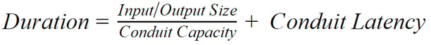
Innoslate can simulate throughput and latency utilizing the Conduit class. A Conduit transfers/transferred by an Input/Output. The simulated delay of an Input/Output is equal to the Size of the Input/Output over the Capacity of the Conduit which transfers the Input/Output plus the Latency of the Conduit. This is expressed in the equation below:
For example, if the Input/Output Size is 20, the Conduit Capacity is 5, and the Conduit Latency is 2 hours the duration will be as follows.
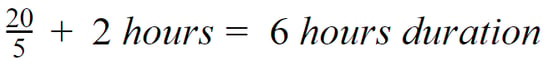
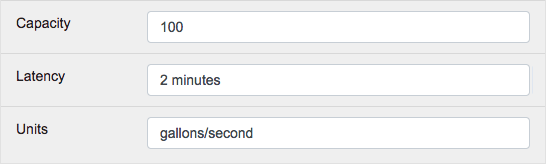
The time units of the Input/Output Size over Conduit Capacity conversion will default to hours. The simulator can also automatically convert and calculate units by utilizing the time units following a slash (“/”) in the Conduit’s Unit attribute. If the time units equal “s” or “sec” or “seconds” then the delay units will equal seconds. If the time units equal “m” or “min” or “minutes” then the delay units will be equal to minutes. If there is no slash (“/”) or the time units are not understood, the time units will be hours. For example, if the Conduit Latency is 1 minute, the Conduit Capacity is 100, the Conduit Units are gallons/second, and the Input/Size is 500 then the resultant Duration will equal 65 seconds (500/100 seconds + 1 minute).
Note: If an Input/Output is transferred by multiple Conduits the simulator will output a warning message to the ‘Console’ panel.
Cloning
Cloning creates copies of an existing Action and its decomposition at simulation run-time. The simulator will copy an Action and execute each copy as if each copy was its own parallel branch. The number of clones can be set by modifying the decomposes/decomposed by Multiplicity relationship attribute. To set this attribute select the Action to be cloned in the ‘Action Diagram’ and click the ‘Open’ drop-down and then select the ‘Entity View’ menu item to navigate to the Action’s ‘Entity View.’ Then click the ‘Attributes’ button under the decomposes/decomposed by relationship. Set the relationship’s Multiplicity attribute to the number of clones desired.
Cost
Total Cost will be automatically calculated based on the incurs/incurred by relationship to Assets or Actions during a simulation run. A Cost’s Amount is added to the simulation’s total running costs. If an entity has multiple incurs Cost relationships the simulator will add the costs individually.
The simulator can calculate “Fixed” or “Per Hour” costs by setting the ‘Rate’ attribute. If ‘Rate’ equals “Fixed” then the cost will be added to the simulation’s cost at the value specified regardless of the duration of the associated model element. If ‘Rate’ equals “Per Hour” then the Cost’s Amount will be multiplied by the duration of the model element. Below is the equation representation of this.
![]()
Note: The Units of the first Cost the simulator encounters will be used as the units for that simulation run.
Wait States
The simulator panels utilize colors to identify the Action’s state during simulation. The table below identifies each state and its appropriate color.
| Color | State | Description |
|---|---|---|
| Gray | Inactive | The Action was not activated or has been killed by a SYNC point. |
| Yellow | Input/Output Wait | The Action is waiting for an Input/Output(s). |
| Purple | Resource Wait | The Action is waiting for a Resource Amount(s). |
| Orange | Asset Utilization Wait | The Action is waiting for enough Asset performers to execute. |
| Maroon | Cloning Operation | The Action is currently being executed through a cloning operation. |
| Green | Executing | The Action is currently executing. |
| Blue | Complete | The Action has completed execution. |
To continue learning about Simulators, Click Here.
(Next Article: Innoslate Scripting Guide)